When working with Excel often, it is extremely useful to freeze columns in excel or rows. As a result, you can easily manage data and work in a simple and effective way. The following article will show you how to freeze columns in Excel 2007.
If you are a person who works regularly with Excel, then fixing important columns will be very useful for you, helping you manage lists, tables, statistics easily and professionally.
Guide to freeze columns in Excel
To freeze columns in Excel 2007, do the following:
Method 1: Freeze only the first column
Step 1: On the Excel toolbar, open the View tab, select Freeze Panes .
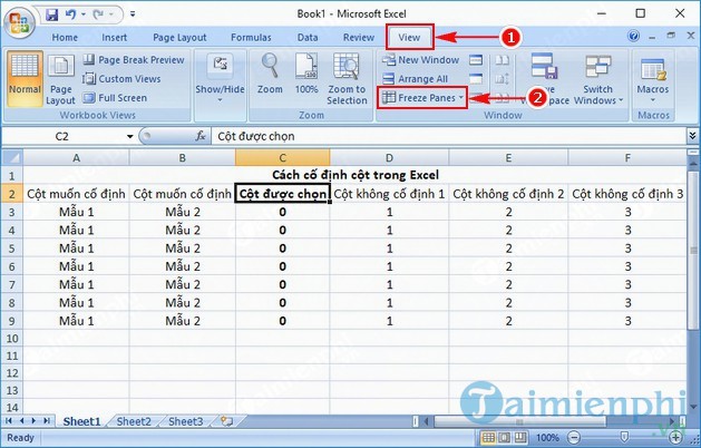
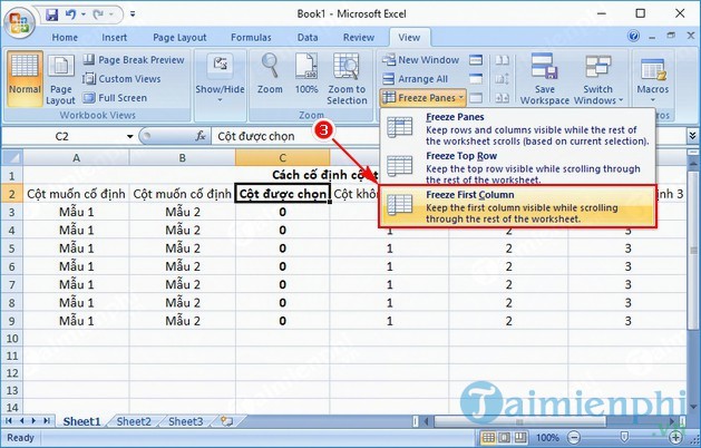
Step 2: For Freeze Panes , select Freeze First Column .
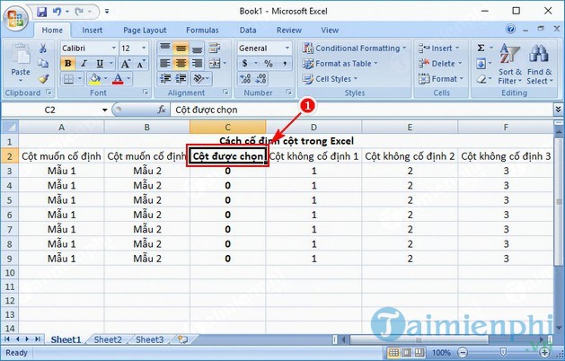
So you can freeze the first column to your Excel file.
If you want to freeze more columns, do as you do in method 2.
Method 2: Freeze multiple columns
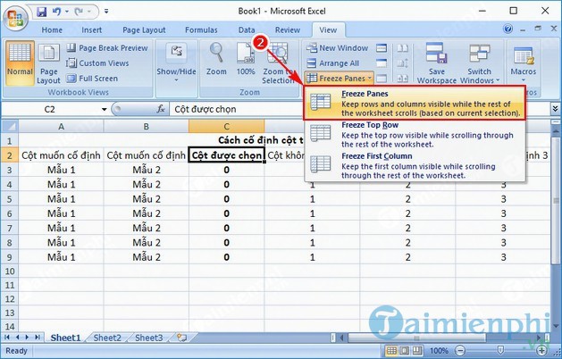
Step 1: Locate the column to be fixed.
Select the first cell of the column to the right of the column to be fixed (because the columns to the left of the selected column will all be fixed).
Step 2: Open the View tab, select Freeze Panes . Select Next Freeze Panes .
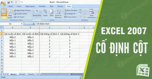
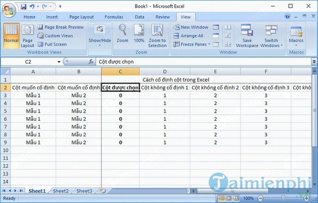
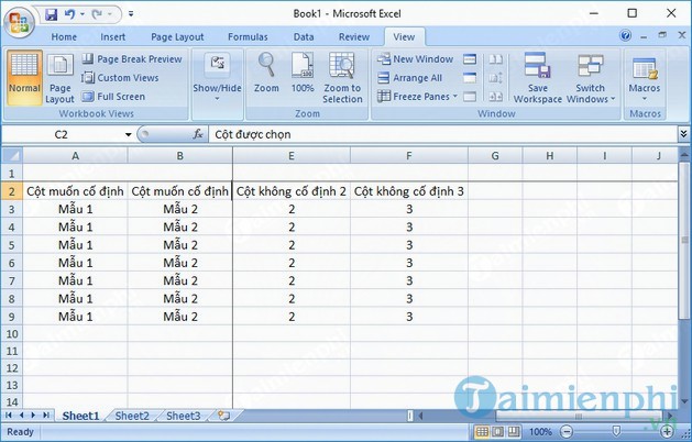
As you can see in the image below, the first 2 columns of the table are fixed.
Before freezing columns
After fixing columns
Above we have done showing you how to freeze columns in Excel. In addition, you can refer to the article how to:
https://thuthuat.taimienphi.vn/cach-co-dinh-cot-trong-excel-35419n.aspx
Besides, when manipulating excel spreadsheets, when 1 line has too much data to enter, you need to do a line down operation in Excel or a line break to make the tool easier to see, if you do not know how to do it, you follow how